Stratified sampling

12 Jun 2021

What is stratified sampling?

Suppose we have to carry out a nation wide survey in India. Since there are more than a billion people, we decide to interview only 10,000 Indians. We can either randomly choose our potential respondents or choose them based on some other factor. For example, if the gender of the respondent is an important factor in the survey, then we might want to ensure that both males and females are represented well. To do this, we can look at the gender ratio in the entire Indian population, and maintain the same ratio while choosing our respondents too. In India, 48.04% of the population are females and 51.96% are males. With this knowledge, we randomly pick 4804 (48.04% of 10,000) and 5196 (51.96% of 10,000) females and males respectively from the entire population.

What we have done here is this: we divided the population into two mutually exclusively groups (males and females), and picked randomly from each group. The number of respondents from each group depended on the size of the group with respect to the entire population. This type of sampling is called stratified random sampling. In statistics jargon, the groups are called strata (plural of stratum), and that’s why we have the word ‘stratified’ in the name.

ML example: California housing data set

Let’s come back to our data set on house prices in California. Our task is to predict the median house value in a district. While there are many attributes in the data set, we can guess that median_income of a district strongly influences the house value in that district (districts with higher median incomes have more expensive houses). Therefore, we ideally want every income value that is present in the data set to be represented well in the test set too (just like correctly representing both the genders in the survey we considered above).

However, this is not practical because there are 12,928 unique income values . To deal with this, we group the median income values into five categories, each group representing a range of incomes. We then calculate what percentage of the districts come under each category, and seek to maintain the same distribution in the test set too.

We classify the incomes into five different categories by introducing a new attribute called income_cat. The pd.cut() method groups a set of values into different categories. The group labels – 1, 2, 3, 4, 5 – are passed as arguments to the labels parameter.

housing["income_cat"] = pd.cut(housing["median_income"],
                               bins=[0., 1.5, 3.0, 4.5, 6., np.inf],
                               labels=[1, 2, 3, 4, 5])

Here is the distribution of income values across different categories.

Category 1: From 0.0 to 1.5 (excluding 0.0)
Category 2: From 1.5 to 3.0 (excluding 1.5)
Category 3: From 3.0 to 4.5 (excluding 3.0)
Category 4: From 4.5 to 6.0 (excluding 4.5)
Category 5: 6.0 and beyond (excluding 6.0)

We now calculate the percentage share of each income category by dividing the output of pd.value_counts() by the number of entries in the data set. value_counts() method gives the number of values in each income category.

housing["income_cat"].value_counts() / len(housing)

The output below shows the percentage distribution of districts across different income categories. We see that 35% of the districts come under income category 3, and categories 2 and 3 together account for about 67% of the districts.

Output:

Now, our task is to split the full data set into training and test sets such that the above distribution is maintained in the test set too. Since we want to have identical distributions in both of them, we use Stratified sampling.

Stratified sampling using `scikit-learn`

Python’s scikit-learn library provides tools to split a data set into two by by stratified sampling.

from sklearn.model_selection import StratifiedShuffleSplit

split = StratifiedShuffleSplit(n_splits=1, test_size=0.2, random_state=42)
for train_index, test_index in split.split(housing, housing["income_cat"]):
    strat_train_set = housing.loc[train_index]
    strat_test_set = housing.loc[test_index]

StratifiedShuffleSplit is a class defined in the model_selection module of sklearn library. According to its documentation, it ‘provides train/test indices to split data in train/test sets’.

In the code above, we first created an instance of the class StratifiedShuffleSplit, and assigned it to the variable split. In other words, split is a StratifiedShuffleSplit object. The split ratio (20% of the full data set is test set) is passed as a parameter while creating the object. The parameter n_split specifies the number of re-shuffling and splitting iterations. It’s default values is 10, but we have changed it to 1. Passing an integer value to random_state ensures reproducible output across multiple function calls.

split() is a method defined in the class StratifiedShuffleSplit, and hence available to all StratifiedShuffleSplit objects. It returns two numpy arrays containing two sets of indices. The data set is split into two based on these indices.

For example, all indices of entries forming the training set are assigned to the variable train_index. The actual training set is formed by picking the entries corresponding to the indices in train_index. This is accomplished by the pd.loc() method. The training and test sets are assigned to the variables strat_train_set and strat_test_set respectively.

If you are curious, you can print the numpy arrays by running the code given below.

for train_index, test_index in split.split(housing, housing["income_cat"]):
  print(train_index)
  print(test_index)

Note that we have two objects with the same variable name split and they are completely different from each other. The first one is an instance of StratifiedShuffleSplit class, and the second one is a method defined in the StratifiedShuffleSplit class. Also, the first one is an object created by us, and the second one is a predefined function.

Let’s now see how districts are distributed across housing categories in the test set (strat_test_set).

strat_test_set["income_cat"].value_counts() / len(strat_test_set)

Output:

Clealry, the districs are almost identically distributed in full data set and test sets.

How close are the distributions?

We can quantify the difference between the distributions in full and test sets by calculating the percentage error (with respect to distribution in full data set).

To do this, we first define a pretty function to calculate the proportion of districts under each income category. The data set is passed as a parameter.

def income_cat_proportions(data):
  return data["income_cat"].value_counts() / len(data)

The percentage error for each income category is calculated by the the following formula.

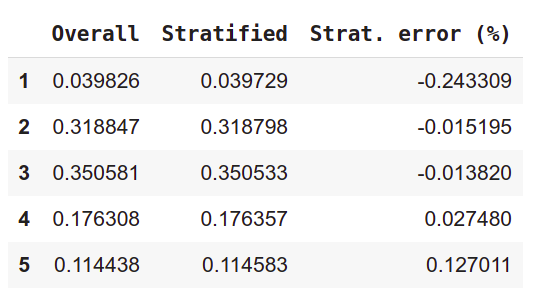
\[\begin{aligned} \% \text { error} &=\frac{\left(\begin{array}{l} \text { Prop. in } \\ \text { test set } \end{array}\right)-\left(\begin{array}{c} \text { Prop. in } \\ \text { full data set } \end{array}\right)}{\text { Prop. in full data set }} \times 100 \\ &=\left(\frac{\begin{array}{l} \text { Prop. in } \\ \text { test set } \end{array}}{\begin{array}{c} \text { Prop. in } \\ \text { full data sit } \end{array}} \times 100\right)-100 \end{aligned}\]

Given below is a crisp code that creates a dataframe of income category proportions, and their corresponding percentage errors for both the full data set and the test set.

compare_props = pd.DataFrame({
    "Overall": income_cat_proportions(housing),
    "Stratified": income_cat_proportions(strat_test_set),
}).sort_index()
compare_props["Strat. error (%)"] = 100 * compare_props["Stratified"] / compare_props["Overall"] - 100

Just printing the dataframe in colab or Jupyter notebook displays the numbers in the form of a nice table. Since the percentage errors are very low, we can conclude that the full data set and the test set have (almost) identical distribution of districts across different income categories.

This is exactly what stratified sampling does - maintain the relative proportions (wrt to the entire population) of subgroups in the sample as well.

percentage error

PS: All the pretty functions in this post are taken from Aurelien Geron’s wonderful book Hands-On Machine Learning with Scikit-Learn & TensorFlow