Probability density function and probability
Consider a microscopic particle that can move only along the \(x-\) axis. The wavefunction that describes the motion of the particle is obtained by solving the Schrodinger equation:
\[\begin{equation} i \hbar \frac{\partial \Psi}{\partial t}=-\frac{\hbar^2}{2 m} \frac{\partial^2 \Psi}{\partial x^2}+V \Psi \label{eq1} \end{equation}\]In Eq.\eqref{eq1}, \(\Psi \equiv \Psi(x, t)\) is the wave function, \(V \equiv V(x,t)\) is the potential energy function describing the environment in which the particle exists, and \(\hbar=\frac{h}{2 \pi}=1.054572 \times 10^{-34} \mathrm{~J} \mathrm{~s}\) is the reduced Planck’s constant.
Wave function (WF) by itself doesn’t tell you anything useful about the particle. In fact, the WF has no physical significance at all. However, once we know the WF, we can answer questions like What is the likelihood of finding the particle between \(x=a\) and \(x=b\) at some time \(t\)?. The answer to this particular question is obtained by solving the integral:
\[\begin{equation} \int_a^b|\Psi(x, t)|^2 \mathrm{d}x. \end{equation} \label{eq2}\]The integrand in eq.\eqref{eq2}, i.e. \(|\Psi(x, t)|^2\) is called the probability density function. The product
\[|\Psi(x, t)|^2 \mathrm{d}x\]is the probability density for finding the particle in an interval of length \(\mathrm{d}x\). For a given \(t\), the probability density function \(|\Psi(x, t)|^2\) is a function of \(x\). Therefore, if we plot \(|\Psi(x, t)|^2\) vs \(x\), we get one curve for each value of \(t\). The figure below shows \(|\Psi(x, t)|^2\) vs \(x\) curves for two different times \(t_{1}\) and \(t_{2}\).
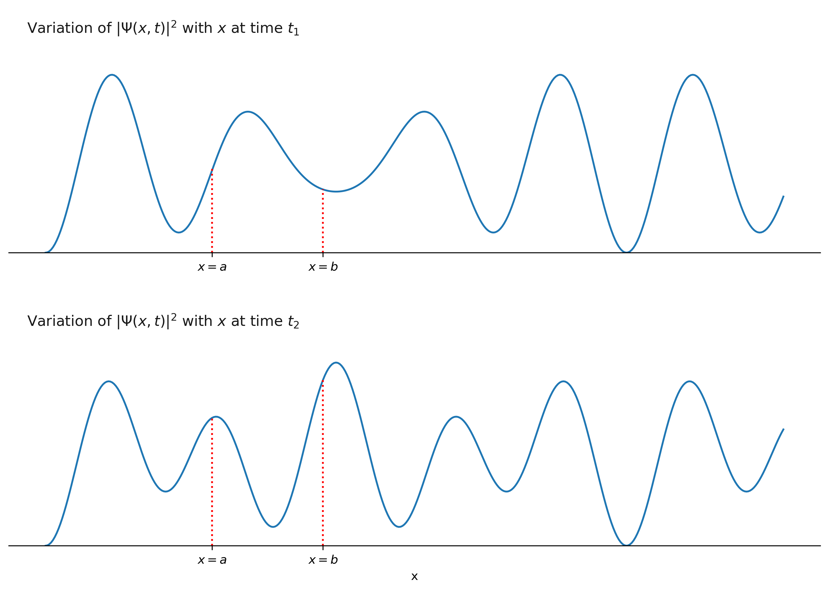
The probabilities of finding the particle between \(x=a\) and \(x=b\) at times \(t_1\) and \(t_2\) are given by:
\[\begin{equation} \int_a^b|\Psi(x, t_{1})|^2 \mathrm{d}x. \end{equation} %\label{eq2}\]and
\[\begin{equation} \int_a^b|\Psi(x, t_{2})|^2 \mathrm{d}x. \end{equation} %\label{eq2}\]respectively. The probabilities are also numerically equal to the areas under the curves (at \(t_{1}\) and \(t_{2}\)) between the points \(x=a\) and \(x=b\). If the areas under the curves (within the same interval) are different at time \(t_{1}\) and \(t_{2}\) are different, then the corresponding probabilities are also different. The value of \(|\Psi(x, t)|^2\) can be greater than 1, but the value of probability can’t exceed 1.
Interestingly, the probability of finding the particle at a given point at a given time is zero. This is because, at \((x, t)\), \(|\Psi(x, t)|^2\) is a point and the integral in eq. \eqref{eq2} vanishes as the upper and lower limits of integration are same.
Normalisation
Though the particle can move only along the \(x-\) axis, it can be anywhere along the axis. Therefore, at any time, it will be somewhere along the \(x-\) axis. In other words, the probability of finding the particle along the \(x-axis\) at anytime is 1. This can be written as:
\[\begin{equation} \int_{-\infty}^{\infty}|\Psi(x, t)|^2 \mathrm{d}x = 1. \label{eq5} \end{equation}\]Equation \eqref{eq5} is often called the normalisation condition. It is a very important condition because only those wave functions that satisfy eq. \eqref{eq5} can represent physical systems. That means, Schrodinger equation can have many solutions but only those solutions that satisfy normalisation condition have physical significance.
The limits of integration in eq. \eqref{eq5} are defined by the problem domain. For example, if the particle is constrained to move between \(x=0\) and \(x=a\), then the normalisation condition is written as:
\[\begin{equation} \int_{0}^{a}|\Psi(x, t)|^2 \mathrm{d}x = 1. \end{equation}\]Normalisation constant
If \(\Psi(x, t)\) is a solution of the Schrodinger equation, then \(A \Psi(x, t)\) is also a solution, where \(A\) is a complex constant. \(A \Psi(x, t)\) represents a physical particle only if it satisfies the normalisation condition:
\[\begin{equation} |A|^{2}\int_{-\infty}^{\infty}|\Psi|^{2} \mathrm{d}x = 1. %\label{eq4} \end{equation}\]The value of \(A\) is obtained by:
\[\begin{equation} |A|^{2}=\left[\int_{-\infty}^{\infty}|\Psi|^{2} \mathrm{d}x\right]^{-1} \label{eq8} \end{equation}\]Here is an interesting question: we know that \(|\Psi(x, t)|^2\) varies with time; does it mean that
\[\begin{equation*} \int_{-\infty}^{\infty}|\Psi(x, t)|^{2} \mathrm{d}x \end{equation*}\]also varies with time?
If that is the case, then the normalisation condition may not be met for every \(t\), and hence the wavefunction may not represent a physical particle at all times. It also means that the value of \(A\) is a function of time. Luckily, it is not the case and it can be shown that,
\[\begin{equation} \frac{d}{dt} \int_{-\infty}^{+\infty}|\Psi(x, t)|^2\, \mathrm{d}x = 0. \label{eq9} \end{equation}\]Equation \eqref{eq9} simply means that the integral in eq. \eqref{eq8} is a constant with respect to time. From this result, we can conclude the following:
- If a wave function is normalisable at \(t=0\), then it remains normalisable for any value \(t\).
- The value of \(A\) is
independent of \(t\). That is, if we find \(A\) at \(t=0\), then it will remain same for any value of t. - For each \(t\), \(|\Psi(x, t)|^2\) vs \(x\) curve can be different but the total area under each curve is same and is equal to 1. However, area under a curve for a given interval can vary with \(t\). Physically, this simply means that the prpbability of finding a particle within an interval varies with time.
A special case
Surprisingly, \(|\Psi(x, t)|^2\) vs \(x\) curve can be same for all values \(t\). But, this can happen only under very special circumstances:
- The potential energy function doesn’t vary with time. i.e. \(V(x,t)\equiv V(x)\)
- The wave function \(\Psi(x, t)\) can be expressed as a product of two functions: \(\Psi(x, t) = \psi(x) \phi(t)\), where \(\psi\) and \(\phi\) are functions of \(x\) and \(t\) respectively.
If a physical system satisfies the above two conditions, then the probability of finding the particle within an interval becomes a constant in time.