Direction cosine matrix
Direction Cosine Matrix (DCM) is the fundamental way we transform between sets of attitude coordinates. For this reason, it’s called the Mother of all Attitude Parameterisations.
Consider two frames \(N\) and \(B\) with relative orientations as shown in figure below.
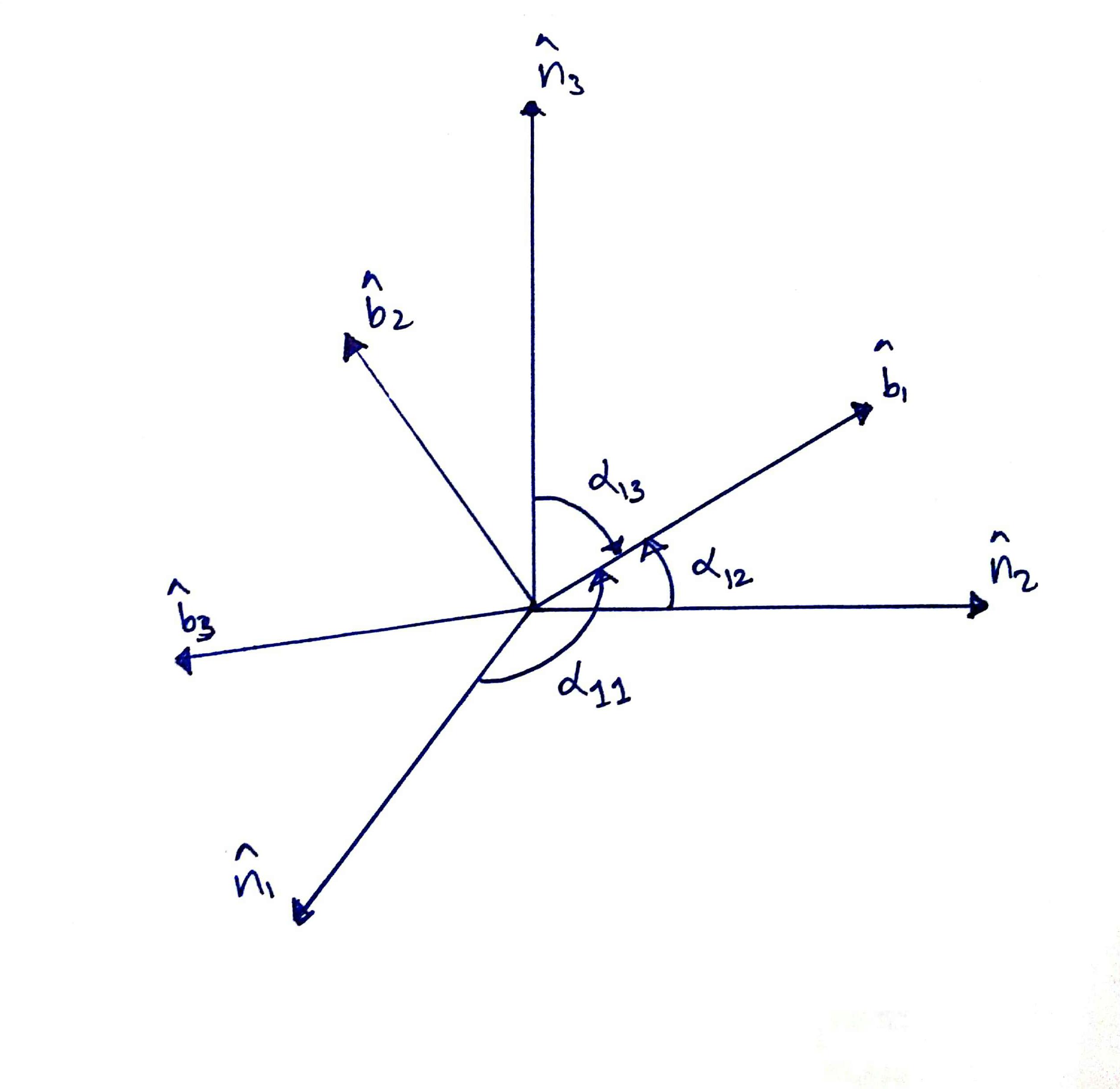
The base vectors \(\mathbf{\hat{\{ b \}}}\) of \(B\) frame can be expressed in terms of base vectors \(\mathbf{\hat{\{ n \}}}\) of \(N\) frame as given below.
\[\begin{align} \hat{\mathbf{b_{1}}} = \cos \alpha_{11}\,\mathbf{\hat{n_{1}}} + \cos \alpha_{12}\, \mathbf{\hat{n_{2}}} + \cos \alpha_{13}\, \mathbf{\hat{n_{3}}} \nonumber \\ \hat{\mathbf{b_{2}}} = \cos \alpha_{21}\, \mathbf{\hat{n_{1}}} + \cos \alpha_{22}\, \mathbf{\hat{n_{2}}} + \cos \alpha_{23}\, \mathbf{\hat{n_{3}}} \label{eq:n2b} \\ \hat{\mathbf{b_{3}}} = \cos \alpha_{31}\, \mathbf{\hat{n_{1}}} + \cos \alpha_{32}\, \mathbf{\hat{n_{2}}} + \cos \alpha_{33}\, \mathbf{\hat{n_{3}}} \nonumber \\ \end{align}\]where \(\alpha_{11}\), \(\alpha_{12}\), and \(\alpha_{13}\) are the angles between \(\mathbf{\hat{b_{1}}}\) and \(\mathbf{\hat{n_{1}}}\), \(\mathbf{\hat{b_{1}}}\) and \(\mathbf{\hat{n_{2}}}\), and \(\mathbf{\hat{b_{1}}}\) and \(\mathbf{\hat{n_{3}}}\) respectively. In general, \(\alpha_{ij}\) is the angle between \(\mathbf{\hat{b_{i}}}\) and \(\mathbf{\hat{n_{j}}}\) vectors, where \(i, j = 1, 2, 3\).
In matrix notation, equation \eqref{eq:n2b} can be written as,
\[\begin{equation} \mathbf{\hat{\{ b \}}} = \begin{bmatrix} \cos \alpha_{11} & \cos \alpha_{12} & \cos \alpha_{13} \\ \cos \alpha_{21} & \cos \alpha_{22} & \cos \alpha_{23} \\ \cos \alpha_{31} & \cos \alpha_{32} & \cos \alpha_{33} \\ \end{bmatrix} \mathbf{\hat{\{ n \}}} = [C]\mathbf{\hat{\{ n \}}}, \end{equation} \label{eq:DCM-n2b}\]where \([C]\) is called the Direction Cosine Matrix (DCM). Elements of the \([C]\) matrix are given by,
\[\begin{equation} C_{ij} = \cos \alpha_{ij} = \mathbf{\hat{b_{i}}} \cdot \mathbf{\hat{n_{j}}}. \end{equation}\]Analogously, mapping from \(B\) to \(N\) is given by,
\[\begin{equation} \mathbf{\hat{\{ n \}}} = \begin{bmatrix} \cos \alpha_{11} & \cos \alpha_{21} & \cos \alpha_{31} \\ \cos \alpha_{12} & \cos \alpha_{22} & \cos \alpha_{32} \\ \cos \alpha_{13} & \cos \alpha_{23} & \cos \alpha_{33} \\ \end{bmatrix} \mathbf{\hat{\{ b \}}} = [C]^\intercal \mathbf{\hat{\{ b \}}}. \end{equation} \label{eq:DCM-b2n}\]Since \([C]\) matrix gives the orientation of \(B\) frame relative to \(N\) frame, the components of DCM are actually attitude coordinates. DCM contains nine coordinates while just three are sufficient to describe attitude. Therefore, DCM is a highly over parameterised set of attitude coordinates. The remaining six redundant coordinates represent the constraints.
In a DCM, every element has to be a cosine of an angle. Therefore, every element should be in the range [-1, +1].
For the DCM, the inverse is the transpose, and hence DCMs are orthogonal matrices. Also, length of each row and column should be 1.
Orthogonality is a very useful property because, to find the inverse of a DCM all we have to do is to find its transpose.
Combining equations \eqref{eq:DCM-n2b} and \eqref{eq:DCM-b2n}, we get,
\[\begin{align} \mathbf{\hat{\{ b \}}} &= [C]\mathbf{\hat{\{ n \}}} = [C][C]^\intercal \mathbf{\hat{\{ b \}}} \label{eq:five} \\ \mathbf{\hat{\{ n \}}} &= [C]^\intercal \mathbf{\hat{\{ b \}}} = [C]^\intercal [C] \mathbf{\hat{\{ n \}}} \label{eq:six} \end{align}\]From equations \eqref{eq:five} and \eqref{eq:six}, it is evident that,
\[[C][C]^\intercal = [C]^\intercal [C] = [I_{3 \times 3}],\]where \([I_{3 \times 3}]\) is the identity matrix. This proves the fact that the inverse of a DCM is is its transpose.
Two letter notation
Two letter notation mentiones the frames whose relative orientations to each other are described by the DCM. For example, the DCM \([C]\) will be written as \([BN]\) clearly demoting that the matrix is a description of the orientation of the \(B\) frame relative to the \(N\) frame. In this notation, equation \eqref{eq:DCM-n2b} can be written as,
\[\begin{equation} \mathbf{\hat{\{b\}}} = [BN]{\mathbf{\hat{\{n\}}}}. \end{equation}\]Examples of DCMs
The identity matrix,
\[\begin{equation} [C] = \begin{bmatrix} 1 & 0 & 0 \\ 0 & 1 & 0 \\ 0 & 0 & 1 \end{bmatrix} \end{equation}\]is a DCM describing two frames that are perfectly aligned with each other. In other words, it describes zero rotation.
Now consider the matrix,
\[[C] = \begin{equation} \begin{bmatrix} 1 & 0 & 1\\ 1 & 0 & 0\\ 0 & 1 & 1 \end{bmatrix}. \end{equation} \label{eq:not-a-DCM}\]The first row tells us that \(\mathbf{\hat{b_{1}}} = \mathbf{\hat{n_{1}}} + \mathbf{\hat{n_{3}}}\). This implies that the length of \(\mathbf{\hat{b_{1}}}\) is \(\sqrt{2}\), which is not correct because it is a unit vector. Therefore, equation \eqref{eq:not-a-DCM} is not a DCM.
Another interesting DCM is,
\[[C] = \begin{equation} \begin{bmatrix} 1 & 0 & 0 \\ 0 & 0 & 1 \\ 0 & 1 & 0 \end{bmatrix} \end{equation} \label{eq:left-handed}\]Here, note that, \(\mathrm{\hat{b_{1}}} = \mathrm{\hat{n_{1}}}\), \(\mathrm{\hat{b_{2}}} = \mathrm{\hat{n_{3}}}\), and \(\mathrm{\hat{b_{3}}} = \mathrm{\hat{n_{2}}}\). The cross products of the base vectors \(\mathrm{\hat{\{b\}}}\) are give by,
\[\begin{align} \mathrm{\hat{b_{1}}} \times \mathrm{\hat{b_{2}}} = \mathrm{\hat{n_{1}}} \times \mathrm{\hat{n_{3}}} = -\mathbf{\hat{n_{2}}} = -\mathbf{\hat{b_{3}}} \\ \mathrm{\hat{b_{2}}} \times \mathrm{\hat{b_{3}}} = \mathrm{\hat{n_{3}}} \times \mathrm{\hat{n_{2}}} = -\mathbf{\hat{n_{1}}} = -\mathbf{\hat{b_{1}}} \\ \mathrm{\hat{b_{3}}} \times \mathrm{\hat{b_{1}}} = \mathrm{\hat{n_{2}}} \times \mathrm{\hat{n_{1}}} = -\mathbf{\hat{n_{3}}} = -\mathbf{\hat{b_{2}}}. \end{align}\]Clearly, the base vectors \(\mathbf{\hat{\{b\}}}\) form a left handed coordinated system. Therefore, the DCM in equation \eqref{eq:left-handed} can not be included in an attitude description using a right handed system.
Reference
- H Schaub and J Junkins. Analytical Mechanics of Space Systems. Published by American Institute of Aeronautics and Astronautics, Inc